7  Sample size

Sample size calculation is a critical component of most experiment designs.¹ The objective of our sample size calculation is to ensure that – over the long-run² – our experiments have the desired Type I error rates (controlled by the significance level, \(\alpha\)) and Type II error rates (controlled by power, \(1-\beta\)).

To perform sample size calculations we use the concept of a minimum detectable effect (MDE) introduced by Bloom (1995), who defines the MDE as follows:

The minimum detectable effect of an experiment is the smallest effect that, if true, has an X% chance of producing an impact estimate that is statistically significant at the Y level.

X is the statistical power of the experiment for an alternative hypothesis equal to the minimum detectable effect. Y is the level of statistical significance used to decide whether or not a true effect exists.

If we perform a two-sided test, we thus have the following two hypotheses:

\[ \begin{align} &H_0: \tau = 0 \\[5 pt] &H_A: \tau = |\Delta|, \end{align} \]

where \(\Delta\) is the MDE and where we use the absolute value to allow for negative or positive effects, given that we perform a two-sided test.

When following this approach, required sample size of an experiment is given by a version of the following formula (e.g. here): \[ n_v = 2(z_{\alpha/2} + z_{1 - \beta})^2\frac{s^2}{\Delta^2}, \tag{7.1}\]

which shows that required sample size is determined by four factors:

1. The probability of making a Type I error, denoted by \(\alpha\), corresponds to the significance level of the test and has an associated with the upper-tail critical value \(z_{\alpha/2}\) in a two-sided test.

2. The probability of making a Type II error, denoted by \(\beta\), determines the power of the test, \(1-\beta\), and has associated critical value given by \(z_{1 - \beta}\).

3. The standard deviation of the outcome variable, \(s\).

4. The minimal detectable effect size, \(\Delta\).

This formula can be intimidating and confusing, all the more so since there are different and sometimes incorrect versions presented in different articles. Worse, rules of thumbs based on the formula are often misunderstood and misapplied because the underlying logic isn’t understood. The aim of this chapter is to demystify the formula by deriving it from scratch.

7.1 Deriving the sample size formula

There are three ways to derive the formula. Two heuristic approaches and one approach that starts from first principles. All three can help us understand what we are doing more deeply.

7.1.1 Bloom approach³

Figure Figure 7.1 shows the sampling distribution of \(\hat{\tau}^{\text{dm}}\) under the null hypothesis (centered around 0, vertical line A) and under the alternative hypothesis (centered around the MDE, vertical line C).

Figure 7.1: Relationship between the MDE and the standard error of an impact estimate. Created with the help of ChatGPT based on similar figure in Bloom (1995).

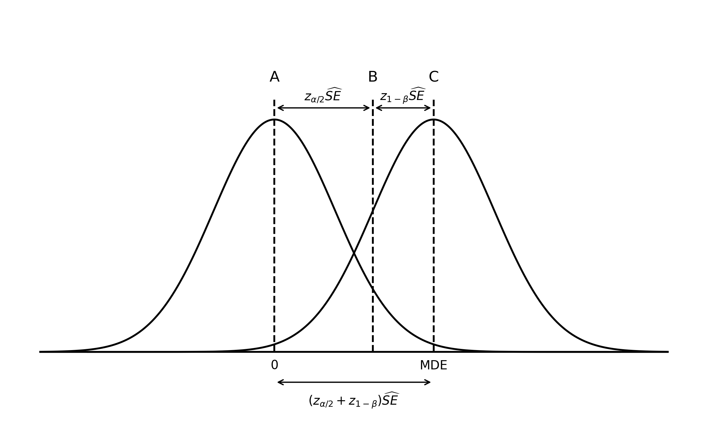
From our hypothesis testing procedure we know that if we want to achieve a Type I error rate of no more than \(\alpha\) we should reject \(H_0\) in a two-sided test on the upper tail if the test statistic, \(t=\frac{\hat{\tau}^{\text{dm}}}{\widehat{SE}}\), falls to the right of the upper-tail critical value \(z_{\alpha/2}\) of the standard normal distribution. That is, we should reject if \(\frac{\hat{\tau}^{\text{dm}}}{\widehat{SE}} > z_{\alpha/2}\). This implies that we should reject the hull hypothesis if, in the sampling distribution, \(\hat{\tau}^{\text{dm}} > \widehat{SE} z_{\alpha/2}\). This threshold for rejection is indicated by vertical line B in the figure. This rejection rule takes care of our Type I error rate.

To ensure adequate power, which will give us our desired Type II error rate, remember that the MDE is defined as the effect size that, if it is true, we have a \(1-\beta\) percent of detecting. In the context of Figure 7.1 this means that if the \(H_A\) distribution on the right hand side is the true distribution, then we have to reject \(H_0\) \(1-\beta\) percent of the time. For this to be true, 80 percent of the mass of the \(H_A\) distribution has to be to the right of the rejection threshold indicated by vertical line B. The distance between that threshold and the center of the \(H_A\) distribution is given by \(z_{1-\beta}\), the critical value in that distribution that has \(1-\beta\) to its right. Having our \(H_A\) distribution positioned in this way takes care of our Type II error rate.

Putting them both together we get: \[ \Delta = (z_{\alpha/2} + z_{1-\beta})\widehat{SE}. \]

7.1.2 Two-equations approach⁴

Collecting the required sample size ensures that (over the course of many experiments), our Type I error rate equals \(\alpha\) and our Type II error rate equals \(\beta\). Instead of directly thinking about the type II error rate, we usually think about it’s complement, power, given by \(1-\beta\).

Using the definition of the MDE above, we know that power is defined for an alternative hypothesis equal to the MDE. If we perform a two-sided test, we thus test the hypothesis:

\[ \begin{align} &H_0: \tau = 0 \\[5 pt] &H_A: \tau = |\Delta|. \end{align} \]

Given our hypothesis testing procedure, ensuring a Type I error that equals \(\alpha\) in a two-sided test requires that:

\[ \frac{\hat{\tau}^{\text{dm}}}{\widehat{SE}} = z_{\alpha/2}. \tag{7.2}\]

Similarly, ensuring a level of power of \(1-\beta\) in a one-sided test requires that:

\[ \frac{\hat{\tau}^{\text{dm}}- \Delta}{\widehat{SE}} = z_{1-\beta}. \tag{7.3}\]

Combining both conditions by rearranging Equation 7.2 for \(\hat{\tau}^\text{dm}\) and substituting that term in Equation 7.3 we get the desired condition: \[ \begin{align} \frac{\widehat{SE}z_{\alpha/2} - \Delta}{\widehat{SE}} &= z_{1-\beta} \\[6pt] \widehat{SE}z_{\alpha/2} - \Delta &= \widehat{SE}z_{1-\beta} \\[6pt] \widehat{SE}z_{\alpha/2} + \widehat{SE}z_{1-\beta} &= \Delta \\[6pt] \widehat{SE}\left(z_{\alpha/2} + z_{1-\beta}\right) &= \Delta. \end{align} \]

7.1.3 First-principles approach

Power is the probability that we reject the null hypothesis if there exists a true effect of size \(\Delta\).

We thus have, for a two-sided hypothesis test: \[ \begin{align} &H_0: \tau = 0 \\[5 pt] &H_A: \tau = |\Delta|. \end{align} \]

We test the null hypothesis by constructing the test statistic \[ t = \frac{\hat{\tau}^{\text{dm}}} {\widehat{SE}}, \]

and reject \(H_0\) if if falls into the rejection region beyond the critical value \(z_{\alpha/2}\). Because the standard normal distribution is symmetric, for a two-sided test we thus reject \(t\) if \[ \begin{align} |t| &> z_{\alpha/2} \\[5pt] \left|\frac{\hat{\tau}^{\text{dm}}}{\widehat{SE}}\right| &> z_{\alpha/2} \\[5pt] \left|\hat{\tau}^{\text{dm}}\right| &> z_{\alpha/2}\widehat{SE}. \end{align} \]

The power \(1-\beta\) of the test under \(H_A\) is the probability that the test statistic \(t\) falls into the rejection region, which is: \[ 1 - \beta = P\left[ \left|\hat{\tau}^{\text{dm}}\right| > z_{\alpha/2}\widehat{SE} \>\middle|\> H_A \right]. \]

The test statistic falling into the lower or upper rejection region are mutually exclusive events, so the above is equal to \[ 1 - \beta = P\left[ \hat{\tau}^{\text{dm}} > z_{\alpha/2}\widehat{SE}\>\middle|\> H_A \right] + P\left[ \hat{\tau}^{\text{dm}} < -z_{\alpha/2}\widehat{SE}\>\middle|\> H_A \right] \]

We can calculate these probabilities by standardising, which gives us:

\[ \begin{align} 1 - \beta &= P\left[ \frac{\hat{\tau}^{\text{dm}} - \Delta}{\widehat{SE}} > \frac{z_{\alpha/2}\widehat{SE} - \Delta}{\widehat{SE}} \right] + P\left[ \frac{\hat{\tau}^{\text{dm}} - \Delta}{\widehat{SE}} < \frac{-z_{\alpha/2}\widehat{SE} - \Delta}{\widehat{SE}} \right] \\[5pt] &= P\left[t > \frac{z_{\alpha/2}\widehat{SE} - \Delta}{\widehat{SE}} \right] + P\left[t < \frac{-z_{\alpha/2}\widehat{SE} - \Delta}{\widehat{SE}} \right] \\[5pt] &= P\left[t > z_{\alpha/2} - \frac{\Delta}{\widehat{SE}} \right] + P\left[t < - z_{\alpha/2} - \frac{\Delta}{\widehat{SE}} \right]. \end{align} \]

Using the standard normal CDF, \(\Phi(z)\), we get:

\[ \begin{align} 1 - \beta =1 - \Phi\left(z_{\alpha/2} - \frac{\Delta}{\widehat{SE}}\right) + \Phi\left(- z_{\alpha/2} - \frac{\Delta}{\widehat{SE}}\right). \end{align} \]

The probability that we reject the null hypothesis for the wrong reason, because the test statistic falls below the lower critical value for a true positive effect or above the upper critical value for a true negative effect, is very small.⁵ Hence, as the true effect size deviates from zero, one of the two terms in the expression above becomes vanishingly small and can be ignored. For the rest of this chapter, I assume we have a true positive effect and omit the second of the two terms above. We thus have:

\[ 1 - \beta = 1 - \Phi\left(z_{\alpha/2} - \frac{\Delta}{\widehat{SE}}\right). \]

Using the symmetry of the standard normal distribution, which implies that \(1 - \Phi(k) = \Phi(-k)\), we can simplify this to

\[ \begin{align} 1 - \beta = \Phi\left(\frac{\Delta}{\widehat{SE}} - z_{\alpha/2}\right). \end{align} \tag{7.4}\]

Next, remember that \(\Phi(z)\) takes z-values and returns probabilities (the probability that a standard normal variable is less than a given z value). The inverse, \(\Phi^{-1}(p)\), thus takes probabilities and returns z-values (the \(z\) value with \(p\) probability mass to its left). Hence, \(\Phi^{-1}(1-\beta)\) refers to the upper-tail critical value of the standard normal distribution that has \(1-\beta\) probability mass to its right, and which we defined above as \(z_{1-\beta}\). Using this, we get:

$$ \[\begin{align} \Phi^{-1}(1 - \beta) &= \Phi^{-1}\left( \Phi\left(\frac{\Delta}{\widehat{SE}} - z_{\alpha/2}\right) \right) \\[5pt] z_{1-\beta} &= \frac{\Delta}{\widehat{SE}} - z_{\alpha/2} \\[5pt] \end{align}\] $${#eq-mde}

Rearranging, we get:

\[ \Delta = \widehat{SE}\left(z_{\alpha/2} + z_{1-\beta}\right). \]

7.1.4 Final step

All three approaches above result in following expression for the MDE:

\[ \Delta = \widehat{SE}\left(z_{\alpha/2} + z_{1-\beta}\right). \]

The final step to get the sample size formula is to plug in the desired version for \(\widehat{SE}\). Depending on the context, we can plug in any of the standard error versions we defined earlier. To arrive at Equation 7.1 from the introduction, we use Equation 5.2, which gives us:

\[ \begin{align} \Delta &= \widehat{SE}\left(z_{\alpha/2} + z_{1-\beta}\right) \\[5pt] \Delta &= \sqrt{\frac{2s^2}{n_v}}\left(z_{\alpha/2} + z_{1-\beta}\right) \\[5pt] \Delta^2 &= \frac{2s^2}{n_v}\left(z_{\alpha/2} + z_{1-\beta}\right)^2 \\[5pt] n_v &= 2\left(z_{\alpha/2} + z_{1-\beta}\right)^2\frac{s^2}{\Delta^2}. \end{align} \]

If, instead of using Equation 5.2 we use the standard error expressed in terms of sample proportions from Equation 5.3, we get: \[ \begin{align} n &= \frac{(z_{\alpha/2} + z_{1-\beta})^2}{p(1-p)} \frac{s^2}{\Delta^2}, \end{align} \] where the left-hand side, \(n\) now refers to the total sample size in the experiment rather than the sample size per variant.

7.2 Rule of thumb

A commonly-used rule of thumb for the required sample size is:

\[ n_v \approx 16\frac{s^2}{\Delta^2}. \] Using Equation 7.1, and the standard critical values \(\alpha = 0.05\) and \(1-\beta = 0.8\), we get: \[ \begin{align} n_v &=2\left(z_{\alpha/2} + z_{1-\beta}\right)^2\frac{s^2}{\Delta^2}\\[6pt] &= 2\left(1.96 + 0.84\right)^2\frac{s^2}{\Delta^2}\\[6pt] &= 15.86\frac{s^2}{\Delta^2}\\[6pt] &\approx 16\frac{s^2}{\Delta^2}. \end{align} \]

Bloom, Howard S. 1995. “Minimum Detectable Effects: A Simple Way to Report the Statistical Power of Experimental Designs.” Evaluation Review 19 (5): 547–56.

List, John A, Sally Sadoff, and Mathis Wagner. 2011. “So You Want to Run an Experiment, Now What? Some Simple Rules of Thumb for Optimal Experimental Design.” Experimental Economics 14: 439–57.

---

1. I say “most” sequential testing approaches do not require ex-ante power calculations.

2. We cannot know significance and power for a single experiment. The best we can do is follow this approach consistently to ensure that over the course of many experiments, they correspond to our desired values. See Chapter 6.

3. This section summarises the approach presented in Bloom (1995).

4. This section is based on List, Sadoff, and Wagner (2011).

5. This type of error is sometimes called a Type III error.